Bring Your Own Data week for TidyTuesday

It’s Bring Your Own Data week for #TidyTuesday, and I decided to analyze my records of events.

I have the habit of recording everything because of my academic jobs. I continue to write down the events I participate in and some interesting information about them. For this exercise, in addition to updating the data with what I did during 2023, I have been cleaning up the data, completing the information, and removing duplicates.

My dataset is a CVS file and has 11 variables. Today we are going to visualize four of them: when the events happened, what format they have (online, in person or hybrid), what role I have (like speaker or organizer) and whay kind of event was (like conference or course).

Plan the visualization

I summarize all the number that I need in differents tibbles and then decide to create a combined plot with:

• the donuts plot that David Schoch use in the GitHub Wrapped project to show general numbers.

• a line plot to show number of events over time.

• a ranked bar plot to show number of events by type and role.

Here is the code:

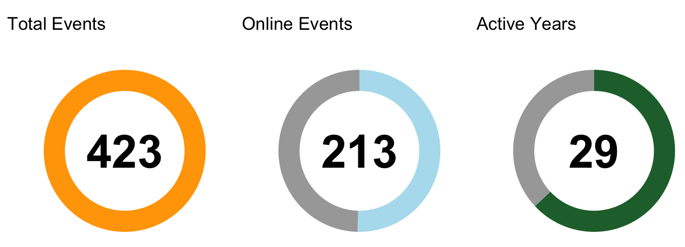
Donuts for Total Numbers

David’s repo have the code of the function donut_plot.

• The total number of events is 423
• The total number of online events is 213 (4 Hybrid and 206 In person).
• The total number of years with records is 29 and I’m 46 years old.

p2 <- donut_plot(423, 423, "orange", "black") + labs(title = "Total Events")
p4 <- donut_plot(213, 423, "lightblue2", "black") + labs(title = "Online Events")
p5 <- donut_plot(29, 46, "#216E39", "black") + labs(title = "Active Years")

This give as result these plots:

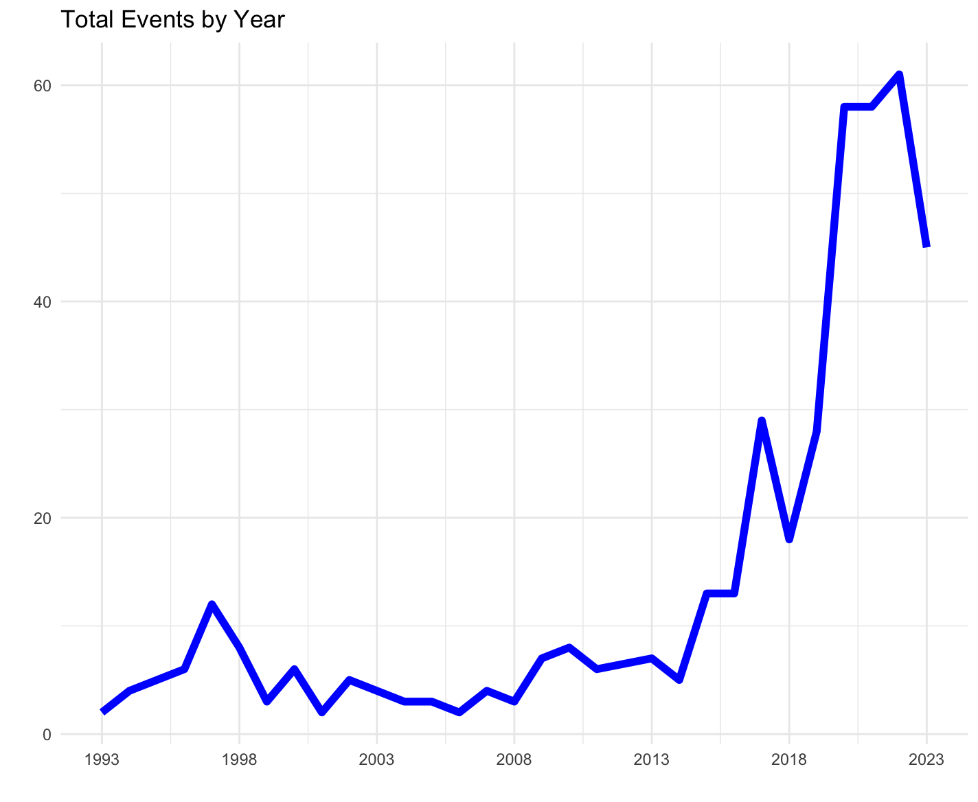
Number of events by year

To show the number of events by year I choose a line plot:

p1 <- totales_year |>
  ggplot(aes(x=anio, y=numero)) +
  geom_line(color = "blue", size=2) +
  labs(title = "Total Events by Year",
       y = "",
       x = "") +
  scale_x_continuous(breaks = c(1993, 1998, 2003, 2008, 2013,2018, 2023)) +
  theme_minimal() 
  

I got this outcome:

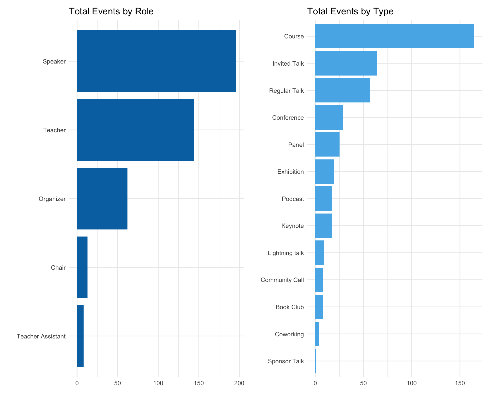
Types of events and roles

Then I plot the bar plots for the type of events and the roles I have in each event. I like ranked plots because helps to visualize the most important categories.

p0 <- totales_rol |>
  ggplot(aes(x=fct_reorder(Rol, numero), y= numero)) +
  geom_col(fill = "#0072B2") +
  coord_flip() +
  labs(title = "Total Events by Role",
       y = "",
       x = "") +
  theme_minimal()

p6 <- totales_tipo |>
  ggplot(aes(x=fct_reorder(Tipo, numero), y= numero)) +
  geom_col(fill = "#56B4E9") +
  coord_flip() +
  labs(title = "Total Events by Type",
       y = "",
       x = "") +
  theme_minimal()

I got this two ranked bar plots with my data by role and by type of events:

Combined plot

Finally, I want to show all of this data together, so I use the package patchwork to create a combined plot with all the preview elements. The code order each of the other plots in the patchwork: first line is all the donuts plots next to each other (p2, p4 y p5), bellow is the line plot (p1), and below it the two bar plot (p0, p6) one next to the other.

(p2 | p4 | p5) / (p1 / (p0 | p6))

This is the final plot:

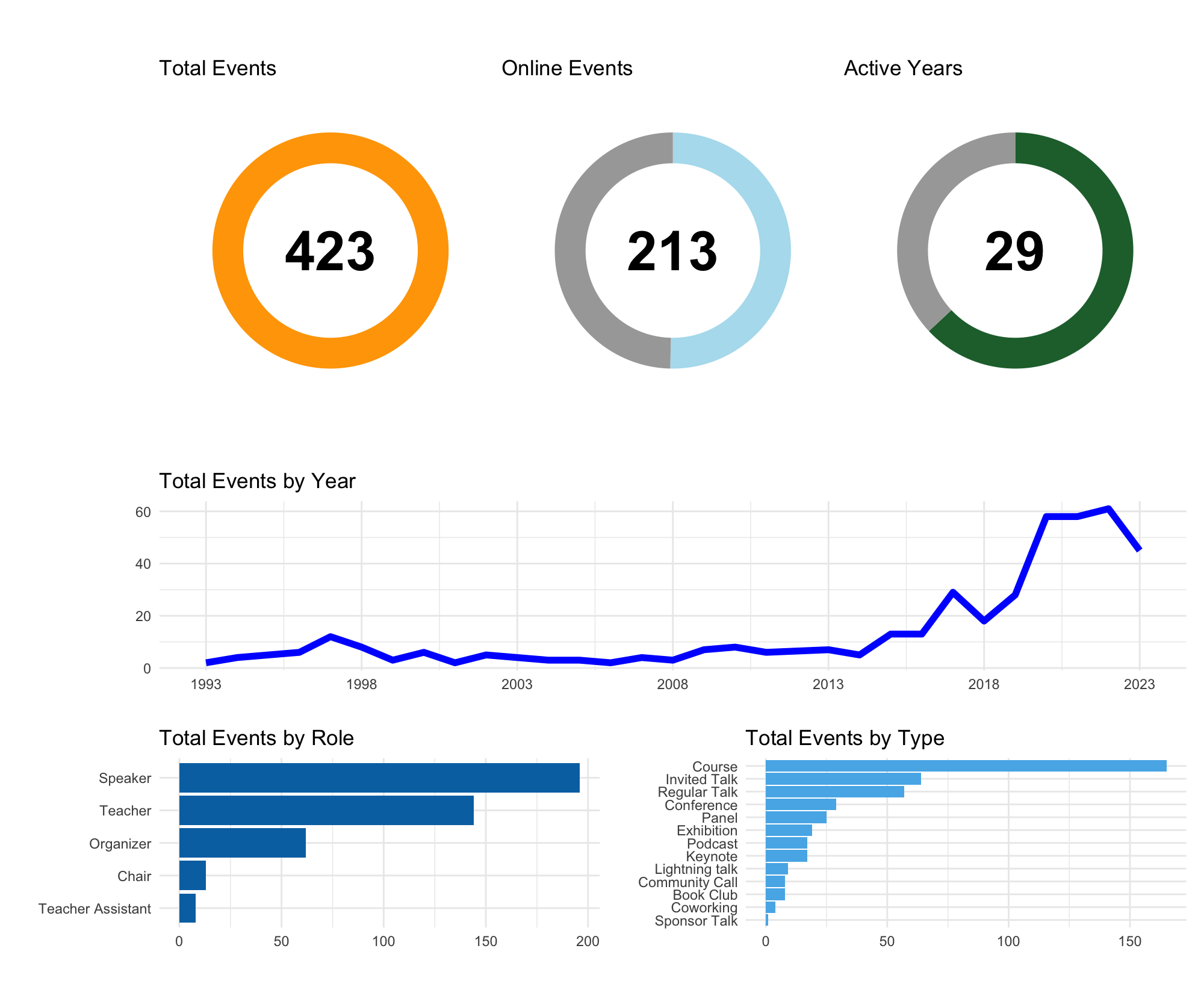
I can improve the annotations for the patchwork, and the disposition of the bar plots, but I kind of like the final output. :-)